… and the Secret of the 90s
Back in 2008, when the hype around Usain Bolt started during the Beijing Olympics, I saw the progression of world records in 100m sprint and found it most curious. For me, it looked like the rate at which world records were achieved had increased in the 90s and I wondered about the reasons behind that. My discussion of these reasons is still valid today, but given that quite some time has passed (2018) and I was a bit sloppy in my initial statistical analysis, I have divided this post into two parts: A) the original discussion from 2008 and B) a more detailed statistical inquiry of my hypothesis that there were suspiciously large improvements in world records starting from the 90s.
A) Intuitions in 2008
During the run-up to the 100m finals in the 2008 Olympics in Beijing the media expressed doubt about the cleanness of the competition (with respect to doping, e.g. [1], [2]). This certainly wasn’t helped by Bolt’s seemingly effortless win which resulted in a new world record on the 100m track [3].
Then I saw a list showing the development of the world records over the 100m from 1912 to now and thought that there are suspiciously many in recent years. So I took that list and made a graph of it:
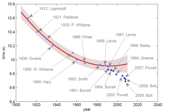
If you look on the development of the world records only until the 80s, it seems that it is following a principle which may be close to the one depicted as a red line. Certainly we can see that the fall of the world record times slowed down. This makes sense, if you assume that there is a natural limit of what a human body can achieve. The red line also suggests that this limit has roughly been hit at the end of the 80s.
But what happened then? In the 90s the world record began to fall further and this development has even picked up since then. Now the world record is falling as quickly as it did in the first half of the 20th century again. So how do we interpret this development? Here are some possible explanations:
- Just a period of slow development in 70s/80s: Between 1936 and 1956 the time for the 100m didn’t decrease much either. Maybe it was the same during the 70s and 80s leading us wrongly to believe that we already hit a limit there. Then we have to ask us why there was no development during that time. Was there no interest in the sport, so not enough new talent came through?
- New training methods: With the help of ever improving training equipment and computer aided analysis based on newest scientific results it is possible to identify and develop athletes’ strengths better than ever before. The question is whether this is enough to explain the drop in world record times. How much of a difference in milliseconds can perfect training methods make? Ultimately it is still the athlete’s body restricting how fast he eventually can run.
- Better development in smaller countries: Maybe new support for sports in non-traditional 100m countries has led to the new fall of world records since the 90s. To some extent the genetics of an athlete determines how fast he can run. That’s what people usually call talent. It seems, for example, that Africans are predestined for long-distance runs. However, as long as there is no proper sports development in the right countries, the talent might stay unrecognised. Jamaica might be one of the countries where new support has created great athletes, but this still doesn’t explain the development in the 90s, because almost all record holders then were American.
- Doping: Finally, what do you do when you have got the talent and excellent training methods and still can’t run any faster, because your body is at its limits? You have to move these limits. Maybe by using substances which increase the level of red blood cells over your natural limit, or let muscles grow stronger than what can be achieved just with training. In this context the plot above suggests that around 1990 athletes started to use doping to push their body limits (and are successful with it) which roughly coincides with when the first doping scandal hit the competition [1].
I know far too little about the development of the sport to make a final judgement about what happened since the 90s. I am convinced that something happened, though, and maybe somebody out there can take it up and clarify more. I certainly believe that there is a limit to how fast a human can run. With doping you might be able to push that limit a bit further. I wonder how far you can eventually go, but I wouldn’t want to test it out. Who knows what happens to your muscles when you have pushed them artificially just a little bit too far? Maybe we should ask one of the record holders in 20 years.
B) Improved statistics in 2018
All of the above discussion was based on the intuition that from about 1970 to 1990 world records in 100m sprint appeared to have converged on a minimum time while from the 90s new world records were produced again. Is it actually possible to find robust statistical support for this hypothesis? This turns out to be a difficult question, because the world record times are only indirect observations of a complicated process. Here I try to characterise this process, I will build a statistical model for it and then evaluate the statistical evidence for my hypothesis. The statistical analysis will demonstrate the use of Gaussian process dynamics in a hierarchical model with censored observations. All analysis code and data is available in my 100m Github repository.
Hidden progression of world performance
My intuition is about a virtual construct that cannot be observed directly: the progression of something I call “world performance” that describes the collective performance across the top athletes at a given time. Even more specifically, I only mean the top performances of the top athletes that are needed to achieve world records. The purpose of my statistical model is to infer this world performance progression from world record times of individual athletes. The basic idea is that the performance of an athlete is a combination of world performance with individual ability and that world records are outstanding top performances of those athletes. I will below go through the corresponding components of the statistical model, but start with a brief description of the data.
World record data
I got the official world records in 100 m sprint from the corresponding Wikipedia page which links to the official results from the IAAF. A complication in the data is that early records were only manually timed with a resolution of 0.1 seconds while from the 1970s more precise automatic timing was introduced. There were 4 automatically timed world records in an overlapping period in which manual and automatic timing co-existed. I rounded these 4 world records down to the nearest .1 second to be compatible with manual times.
Often athletes try to reach their top performance at one major event in a year, e.g., the Olympics. I, therefore, bin world records in yearly bins, but maintain the natural order of world records in the analysis as described below.
World performance dynamics
The crucial part of my analysis was to describe the hidden progression of world performance also in years in which no world records were achieved. Because I didn’t want to make unnecessary assumptions about how world performance changes as a function of time, I assumed that world performance follows a Gaussian process. This states that world performances \(\mathbb{w} = [w_1, \dots, w_n]^T\) at years \(\mathbb{y} = [y_1, \dots, y_n]^T\) are Gaussian distributed
$$\mathbb{w} \sim \mathcal{N}(\mathbb{0}, \Sigma)$$
where \(\Sigma\) is computed by applying a covariance function to the years \(\mathbb{y}\).
Conceptually a Gaussian process describes a probability distribution over functions, here a function from years \(y\) to world performance \(w\). The mentioned covariance function determines the type of functions that can be generated from the Gaussian process. For example, a parameter of the covariance function can determine how smooth the generated functions are. These parameters were inferred together with the world performances \(w\) at all years from 1912 to 2017 in the full model.
Performance of individual athletes
While I assumed that world performance progresses across years, I modeled variability in 100 m times of individual athletes as independent draws from a Gaussian distribution. The mean of that distribution, however, reflects the current world performance in addition to an athlete’s ability in relation to the world performance. In equations:
$$t(a, y) \sim \mathcal{N}\left(w(y) + b_a, \sigma_a\right)$$
where \(a\) identifies an athlete, \(y\) is the current year, \(t(a, y)\) is a 100 m time of athlete \(a\) in year \(y\), \(b_a\) is the athlete’s (mean) ability relative to world performance \(w(y)\) in that year and \(\sigma_a\) is that athlete’s individual variability in performance. The athlete-specific parameters of this distribution, i.e., \(b_a\) and \(\sigma_a\) needed to be inferred from the world record times of each athlete.
It could be that the Gaussian distribution is not the best choice to describe the variability in 100 m times of an athlete, but it was a good start and has limited width of its tails which made it easier to infer the underlying world performance progression. Also, the model I used here targets the virtual entity of world performance that does not really exist and just helps to describe the progression of 100 m world records. It is not crucial for that to find the exact distribution of 100 m times of each athlete. This would also be impossible, because I only tried to model the distribution of only the absolute top of performances in major events for which too few data exist to infer any distribution with high certainty.
Censored data
Data input to the model were the world record times together with their year of achievement and the athlete who achieved it. To get a data point in every year I filled up the data set with data points for each year that had no world record with the last world record time and no athlete. This way the model knew that no athlete achieved a world record in that year.
Every data point tells us that all except the associated athlete did not achieve a world record at the same time, i.e., they only achieved a time that was slower than the time given by the data point (or didn’t compete). This is an instance of censored data and means that the likelihood defined for the data is either based on the probability density of the Gaussian (for the athlete that achieved the world record) or it is based on the cumulative distribution function of the Gaussian (for all other athletes). This is also described in the Stan manual.
Selection of athletes and length of careers
Athletes only perform at their best for a limited period of time. So it is clear that I should not infer anything about Bobby Morrow’s top performances in the 1950s from his inability to achieve a world record in the 1980s. To account for that I limited the influence of individual data points on an athlete’s performance by only including athlete-specific likelihood terms for a limited period of years – the career of an athlete. For all athletes with a world record I defined their career to include all years from 2 years before the year of the first world record to the 6 years after their first world record.
Furthermore, I defined the top athletes in a year to be the 8 athletes that are competing in a typical Olympics final. Because in most years less than 8 world record holders had an overlapping career, I filled up the remaining top athlete spots with anonymous athletes who also had a 9-year long career.
Inference
I implemented the model and data described above in the probabilistic programming language Stan. Bayesian inference in the model is then approximated with Markov chain Monte Carlo sampling. To get inference in this model running reliably was a bit tricky. Because of the many unknowns and little data, priors had to be chosen suitably to allow the sampler to consistently explore the complicated posterior distribution. Results below are based on 2000 samples from the posterior. Details can be found in the Github repository.
Results
The plot below shows the world records of individual athletes as green dots (move the mouse pointer over the points to find out the details of the record). The grey line depicts the progression of the estimated world performance together with a 95% posterior probability interval indicating the posterior uncertainty.
Clearly, the (average) top world performance is above the world records which are extreme events in the model. More importantly, the world performance roughly follows my intuition from above: The line has a roughly linear drop until about 1970, then flattens out to be almost constant and then starts to drop slightly again from 1990. The absence of world records after 2009 again leads to a flattening of the curve that even ends in a small rise from 2016 to 2017. Note that this is expected to happen in long periods without world records, because even for constant world performance world records as extreme events should occur sooner or later. So, if world records do not occur over a long period of time, this is an indicator that the underlying average performance has worsened.
your red line fit is arbitrary and implausible in the first place, you can see it curving up at the end which is goofy. An exponential decay is more reasonable than a parabola
If you re-draw the red line as a steeper hyperbola to take in Bolt’s performances, it may be that Bolt’s record still remains as an outlying point and the imaginary/theoretical point at the bottom/end of the curve in the future remains just that – theoretical and never reached.
The most important statistic in the 100 meter is the timing and speed of the athlete at 10 meter intervals. Sprinters (male) reach top speed around the halfway point and then decelerate. The secret to the modern era in the 100 meter is speed maintenance in the last 40 meters. To this end I believe Bolt is successful due to his size and in particular his leg length. Carl Lewis also had long legs. This provides the sprinter with a higher gear to not lose speed. Thus the proper analysis could be to consider the length of the sprinters stride and how many steps are taken throughout the race and when. I have seen interesting interval charts which demonstrate this point.
To this end I would note that Bolt only took 41 strides in his world record while most others are 43-48 strides. If you want a math formula try stride length by stride frequency. Size matters!
Oh, and tell the athletes to save their celebration until AFTER they cross the finish line. Yes I’m looking at you Mr Bolt.